Methodology Sewage
The methodology combines different open data sources and generates a generic network by open-source technology [34]. The generic network designed by algorithm matches the real sewage network to a certain extent. Therefore, the generic network makes it possible to spot suitable locations for exploitation of waste heat from sewers without having the original GIS data of the sewer. Overall, the methodology allocates population density to street networks and calculates the wastewater volume flow (WWV) for each street. WWV results from the product of population density (PD) and the country-specific water usage (WU) (2.1). Finally, an algorithm determines the shortest paths from each street to the wastewater treatment plant. Furthermore, it accumulates the wastewater volume flows along these paths that are distinguished by residential buildings (discharging waste water at 18 °C), commercial buildings (discharging waste water at 22 °C) and industrial buildings (discharging waste water at 35 °C).
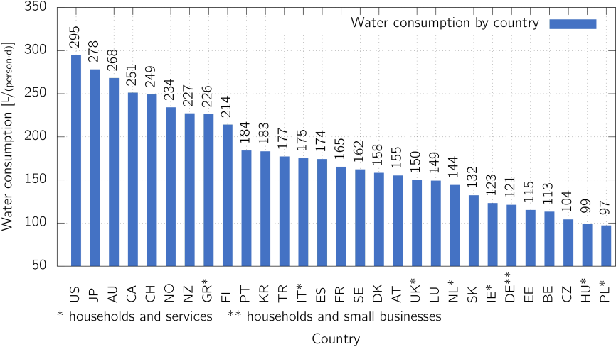
Figure 1: Overview of water consumption by country
The methodology assumes the following:
- Water consumption is equivalent to the amount of wastewater.
- Specific water consumption is the statistical average at national level.
- Rainwater accumulates discontinuously and is therefore neglected.
- The path of the sewage system is said to be the shortest path along the street network from wastewater occurrences to the wastewater treatment plant. Obstacles (e.g. rivers, bridges, train tracks), pumps, geodesic heights are not taken into account.
- Buildings without information on their usage or without fitting key metrics (Fig. 1, Fig. 2 and Fig. 3) on the discharged wastewater will be impinged by the difference between the amount of the calculated wastewater and the waste water published by “GIS Reference Layers on UWWT Directive Sensitive Areas. Description of dataset and processing (ed European Topic Centre Inland, coastal, marine waters)
- 2013” which compiles the wastewater quantities for all wastewater treatment plants throughout the EU and can be accessed by https://www.eea.europa.eu/data-and-maps/data/waterbase-uwwtd-urban-waste-water-treatment-directive-9/documentation/uwwtd_gis_reference_v4/download.
- The heat transfer coefficient is taken into account relating to the pipes diameter given in two ranges and defined by the volume flow in each pipe. The lower range takes average heat transfer coefficient of PET pipes. The higher range assumes heat transfer coefficient of concrete.
The methodology uses graph theory and creates an undirected and unweighted graph out of open-source data. Altogether, the Modell consist of 4 steps:
- M1 Determining the flow direction in the edges of the graph,
- M2 Defining the mass flow in all edges for the three building use categories by allocating the amount of waste water to each building by key metrics and above given discharge temperature,
- M3 Determining the composition of the wastewater flows and the temperatures in each edge and node based on defined flow directions,
- M4 The fourth model optimizes the wastewater waste heat extraction points: it determines the locations, the amount of waste heat and the resulting waste heat temperature.
Each model is solved by using the solver GUROBI and the python package gurobipy. Further information and the systems of equations can be found in the final report at https://www.iea-dhc.org/the-research/annexes.
|
|
|
|
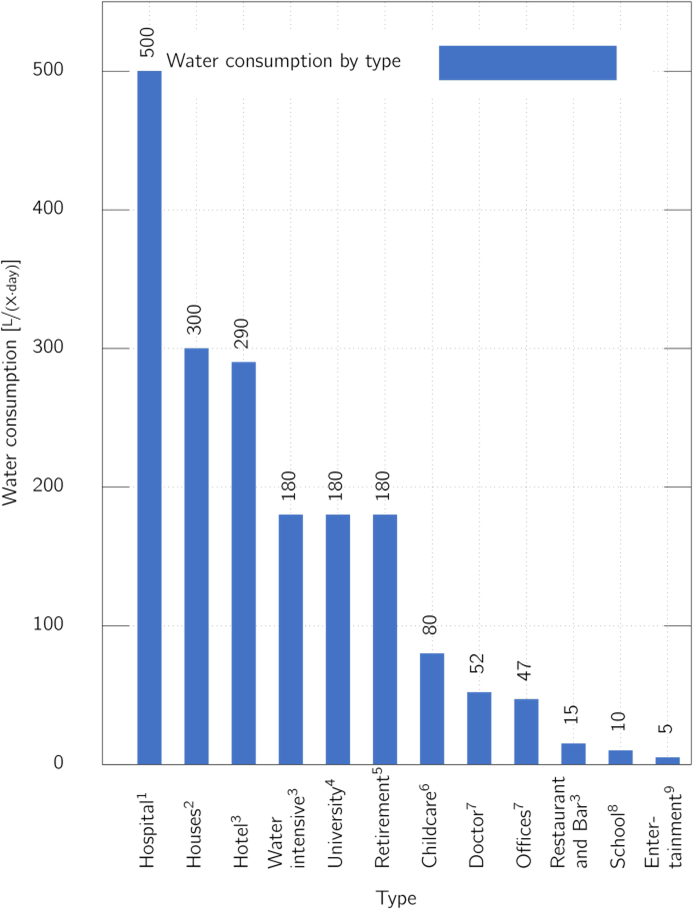
Figure 2: Water consumption by different building types. The amount of water usage depends on the reference value x. (1 x = bed, 2 x = person, 3 x =guest, 4 n.a., 5 x = patient + personell, 6 x = child, 7 x = employee, 8 x = pupil, 9 x = seat) |
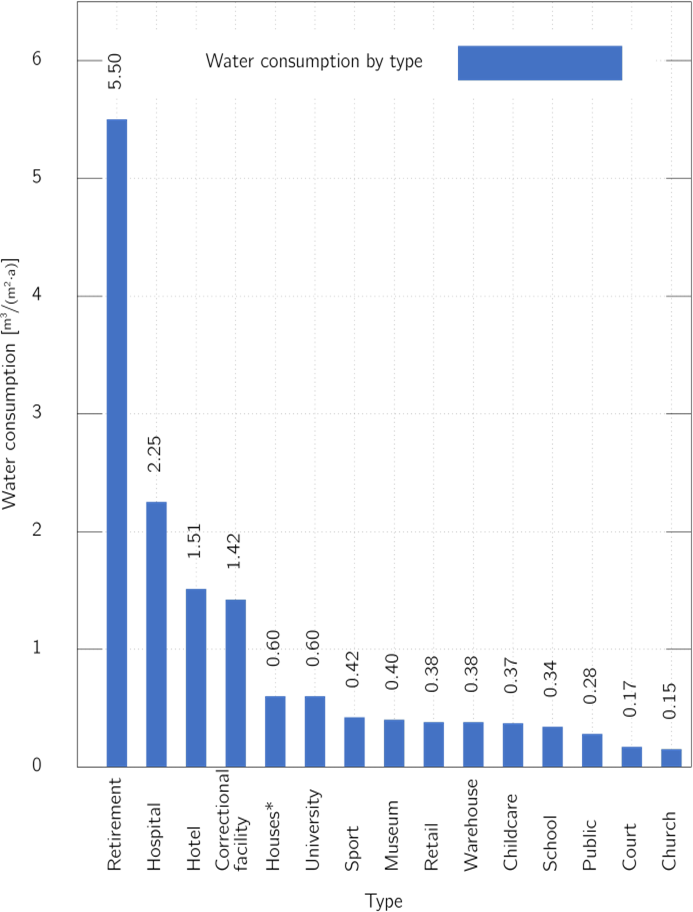
Figure 3: Water consumption by different building types (* used during daytime) |